import numpy as np
from scipy.stats import poisson
from scipy.stats import expon
import matplotlib.pyplot as plt
from IPython.display import Image, display
import seaborn as sns

# Apply the default theme
sns.set_theme()

Exercise

Exercise 1 - Frequentist Upper Limit on a Poisson Parameter

Consider the scenario where the observed count n follows a Poisson distribution:

\[ n \sim \text{Poisson}(s + b) \]

Given that the background expectation is b = 4.5 and the observed count is \(n_{\text{obs}} = 5\) , determine the 95% confidence level (CL) upper limit on s.

Hint

How does the distribution of n change as you vary s?

Exercise 2 - Maximum Likelihood Estimator for a Gaussian Distribution

Suppose individual measurements \(x_i\) are distributed around an unknown true value \(\theta\) according to a Gaussian distribution with a known standard deviation \(\sigma_i\). The probability density function (PDF) is given by:

(1)\[f (x_i;\theta, \sigma_i) = \frac{1}{\sqrt{2\pi}\sigma_i} e^{-\frac{(x_i - \theta)^2}{2\sigma_i^2}}\]

The corresponding log-likelihood function is:

(2)\[\ln L(\theta) = -\frac{1}{2} \sum_{i=1}^{N} \frac{(x_i - \theta)^2}{\sigma_i^2} + \text{constant}.\]

This function describes a parabola, which reaches its maximum at some value \(\hat{\theta}\). Derive the expressions for the maximum likelihood estimator \(\hat{\theta}\), and its uncertainty \(\sigma_{\hat{\theta}}\).

Exercise 3 - Parameter Estimation for Exponential Decay

The probability density function (PDF) for observing a decay at time \(t\) is given by:

(3)\[f (t;\tau) = \frac{1}{\tau} e^{-\frac{t}{\tau}}\]

The goal is to estimate the parameter \(\tau\), which represents the lifetime of the decay. Three different datasets, each containing a different number of events, are provided. Using the maximum likelihood estimation (MLE) method, calculate \(\hat{\tau}\) and \(\sigma_{\hat{\tau}}\) for each dataset and compare the results with those obtained using the Gaussian estimator.

Note

For any probability density function \(f(x;\theta)\), as the number of observed events increases, the likelihood function \(L\) asymptotically approaches a multivariate Gaussian distribution.

# set the random seed
np.random.seed(0)

Ns = [2, 8, 20]
true_tau = 1 
# generate the data
toys_expon = [expon.rvs(size=N, scale=true_tau) for N in Ns]

Exercise 4 - Neyman Construction

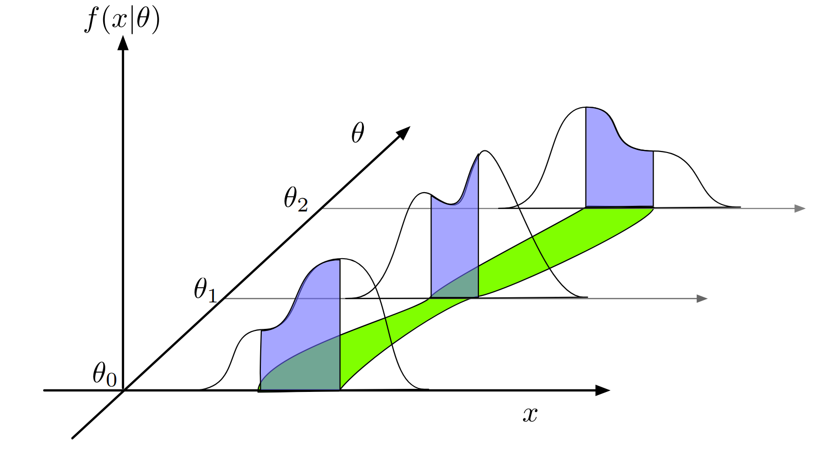
mu = 1
n_s = 5
n_b = 4.5
n_hypo = mu * n_s + n_b

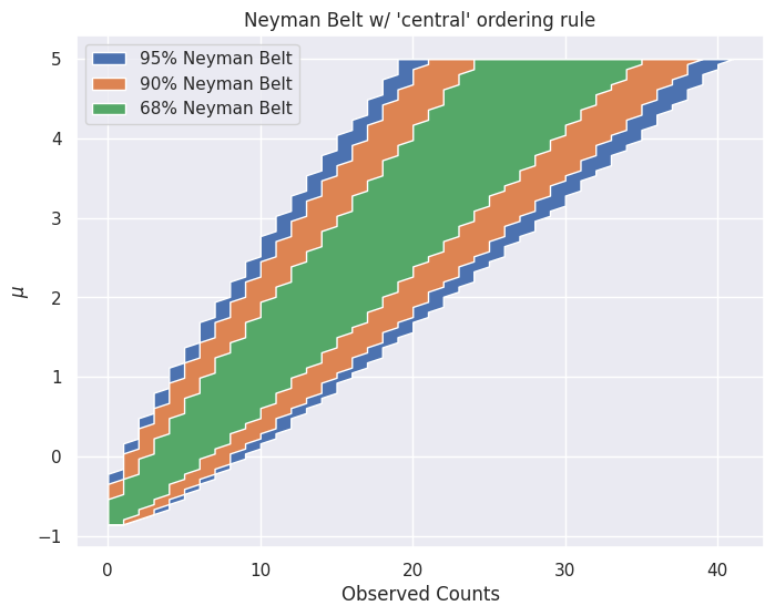
CL_s = [0.68, 0.90, 0.95]
ordering_rules = ["central"]
n_plots = len(ordering_rules)
mus = np.linspace(-2, 5, 111)


fig, axs = plt.subplots( nrows=1, ncols=n_plots, figsize=(8 * n_plots, 6))
for i, ordering_rule in enumerate(ordering_rules):
    ax = axs[i] if n_plots > 1 else axs
    for CL in CL_s[::-1]:
        n_hypo = mus * n_s + n_b

        size = (1 - CL) / 2 if ordering_rule == "central" else (1 - CL)

        lower_bound = poisson.ppf(size, n_hypo) if ordering_rule == "central" else np.zeros_like(n_hypo)
        upper_bound = poisson.isf(size, n_hypo)

        ax.fill_betweenx(mus, lower_bound, upper_bound,
                        label=f"{int(CL*100)}% Neyman Belt")

    ax.set_title(f"Neyman Belt w/ '{ordering_rule}' ordering rule")
    ax.set_xlabel("Observed Counts")  
    ax.set_ylabel(r"$\mu$")           
    ax.legend()
    ax.grid(True)
plt.show()

Pyhf

import pyhf
from pyhf.contrib.viz import brazil
import numpy.random as random
random.seed(0)
pyhf.set_backend("numpy")

model = pyhf.simplemodels.uncorrelated_background(
    signal=[10.0], bkg=[50.0], bkg_uncertainty=[np.sqrt(50)]
)
observations = [60]
data = observations + model.config.auxdata

print(f"  channels: {model.config.channels}")
print(f"     nbins: {model.config.channel_nbins}")
print(f"   samples: {model.config.samples}")
print(f" modifiers: {model.config.modifiers}")
print(f"parameters: {model.config.parameters}")
print(f"  nauxdata: {model.config.nauxdata}")
print(f"   auxdata: {model.config.auxdata}")

  channels: ['singlechannel']
     nbins: {'singlechannel': 1}
   samples: ['background', 'signal']
 modifiers: [('mu', 'normfactor'), ('uncorr_bkguncrt', 'shapesys')]
parameters: ['mu', 'uncorr_bkguncrt']
  nauxdata: 1
   auxdata: [np.float64(49.99999999999999)]

init_pars = model.config.suggested_init()
par_bounds = model.config.suggested_bounds()
fixed_params = model.config.suggested_fixed()

poi_values = np.linspace(0.1, 5, 50)
obs_limit, exp_limits, (scan, results) = pyhf.infer.intervals.upper_limits.upper_limit(
    data, model, poi_values, level=0.05, return_results=True
)
print(f"Upper limit (obs): μ = {obs_limit:.4f}")
print(f"Upper limit (exp): μ = {exp_limits[2]:.4f}")

Upper limit (obs): μ = 2.8447
Upper limit (exp): μ = 2.0751

fig, ax = plt.subplots()
fig.set_size_inches(10.5, 7)
ax.set_title("Hypothesis Tests")

artists = brazil.plot_results(poi_values, results, ax=ax)

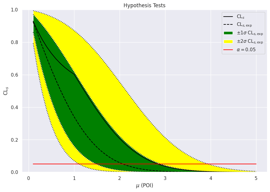
How is this related to the reported upper limits?

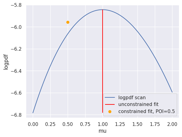
log pdf scan

mu_s = np.linspace(0, 2, 201).reshape(201,1)
test_pars = np.concatenate((mu_s, np.ones_like(mu_s)), axis=1)

logpdf_scan = []
for test in test_pars:
    logpdf_scan.append(model.logpdf(pars=test, data=data))
    

plt.plot(mu_s, logpdf_scan, label="logpdf scan")

uncontrained_fit, uncontrained_fitted_value = pyhf.infer.mle.fit(data=data, pdf=model, return_fitted_val=True)
constrained_fit, contrained_fitted_value = pyhf.infer.mle.fixed_poi_fit(poi_val=0.5, data=data, pdf=model, return_fitted_val=True)
plt.vlines(uncontrained_fit[0], ymin=np.min(logpdf_scan), ymax=np.max(logpdf_scan), label="unconstrained fit", color="red")
# plt.scatter(uncontrained_fit[0], uncontrained_fitted_value, label=f"unconstrained fit")
plt.scatter(constrained_fit[0], model.logpdf(pars=constrained_fit, data=data), label=f"constrained fit, POI={constrained_fit[0]}", color="orange")

plt.xlabel('mu')
plt.ylabel('logpdf')
plt.legend()
plt.show()

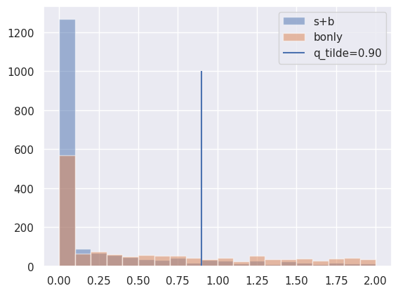
upper limits

mu_test = 1.0

toy_calculator = pyhf.infer.calculators.ToyCalculator(
    data, model, ntoys=2000, track_progress=False, test_stat="qtilde"
)

q_tilde = toy_calculator.teststatistic(2 * mu_test)
sig_plus_bkg_dist, bkg_dist = toy_calculator.distributions(mu_test)

bin_edges = np.linspace(0, 2, 21)
plt.hist(sig_plus_bkg_dist.samples, bins=bin_edges, label="s+b", alpha=0.5)
plt.hist(bkg_dist.samples, bins=bin_edges, label="bonly", alpha=0.5)
plt.vlines(q_tilde, 0, 1000, label=f"q_tilde={q_tilde:.2f}")
plt.legend()
plt.show()

Observed Upper Limit

CLsb, CLb, CLs = toy_calculator.pvalues(q_tilde, sig_plus_bkg_dist, bkg_dist)
CLsb, CLb, CLs

(array(0.1715), array(0.488), array(0.35143443))

print(sum(sig_plus_bkg_dist.samples > q_tilde) / len(sig_plus_bkg_dist.samples))

0.1715

sum(bkg_dist.samples > q_tilde) / len(bkg_dist.samples)

np.float64(0.488)

Expected Upper Limit

CLsb_exp_band, CLb_exp_band, CLs_exp_band = toy_calculator.expected_pvalues(sig_plus_bkg_dist, bkg_dist)

CLsb_exp_band

[array(0.002), array(0.025), array(0.17775), array(1.), array(1.)]

CLb_exp_band

[array(0.0235), array(0.16), array(0.50125), array(1.), array(1.)]

[CLsb / CLb for CLsb, CLb in zip(CLsb_exp_band, CLb_exp_band)]

[np.float64(0.0851063829787234),
 np.float64(0.15625),
 np.float64(0.3546134663341646),
 np.float64(1.0),
 np.float64(1.0)]

CLs_exp_band

[array(0.10606061), array(0.16272189), array(0.35569106), array(1.), array(1.)]

test unc size

import ipywidgets as widgets
@widgets.interact(bkg_unc=(1.0, 20.0, 0.5))  # bkg unc in [0, 10]
def test_unc_size(bkg_unc = 1.0):
    model = pyhf.simplemodels.uncorrelated_background(
        signal=[10.0], bkg=[50.0], bkg_uncertainty=[bkg_unc]
    )

    observations = [60.0] + model.config.auxdata
    poi_values = np.linspace(0.1, 5, 50)
    obs_limit, exp_limits, (scan, results) = pyhf.infer.intervals.upper_limits.upper_limit(
        observations, model, poi_values, level=0.05, return_results=True
    )
    print(f"Upper limit (obs): μ = {obs_limit:.4f}")
    print(f"Upper limit (exp): μ = {exp_limits[2]:.4f}")

    fig, ax = plt.subplots()
    fig.set_size_inches(10.5, 7)
    ax.set_title("Hypothesis Tests")

    artists = brazil.plot_results(poi_values, results, ax=ax)